Differential Gene Expression when dealing with two treatment conditions
Last updated on 2025-12-02 | Edit this page
Overview
Questions
- How do conserved markers help us label clusters reliably across conditions?
- What exactly do avg_log2FC, pct.1, pct.2, and p_val_adj mean in FindMarkers?
- Why must DE be run within a cell type (e.g., CD16 Mono_STIM vs CD16 Mono_CTRL) rather than “all cells”?
Objectives
- Use FindConservedMarkers() to pick markers and label clusters.
- Set identities to annotations and create compound identities (celltype.and.stim) for clean contrasts.
- Run FindMarkers() to get DEGs between conditions within a cell type and interpret key columns.
- Visualize DEGs (FeaturePlot with split.by, DoHeatmap / pheatmap) and export results for downstream use.
- Recognize pitfalls (composition effects, inappropriate contrasts, overly lenient thresholds).
OUTPUT
Modularity Optimizer version 1.3.0 by Ludo Waltman and Nees Jan van Eck
Number of nodes: 13548
Number of edges: 521570
Running Louvain algorithm...
Maximum modularity in 10 random starts: 0.9002
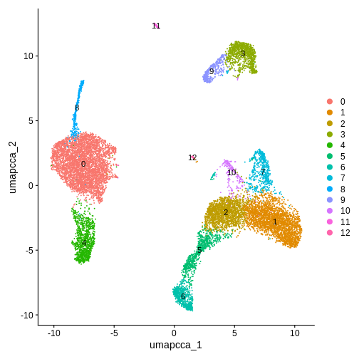
Number of communities: 13
Elapsed time: 2 secondsR
DimPlot(ifnb.filtered, reduction = "umap.cca", label = T)
R
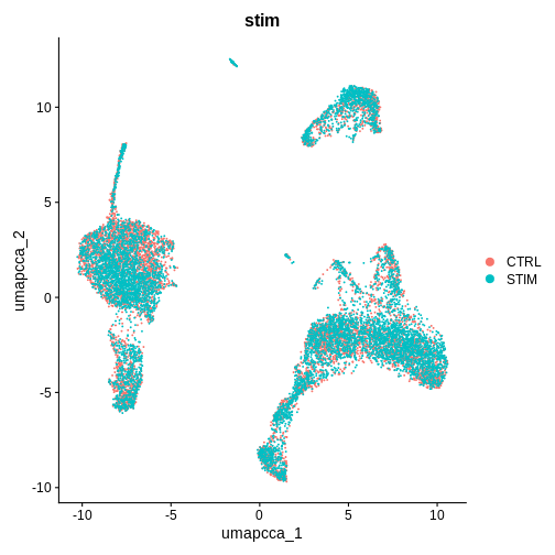
DimPlot(ifnb.filtered, reduction = "umap.cca", group.by = "stim")
Step 1. Find Conserved Markers to label our celltypes
R
## Let's look at conserved markers in cluster 4 across our two conditions (compared to all other clusters)
markers.cluster.4 <- FindConservedMarkers(ifnb.filtered, ident.1 = 4,
                     grouping.var = 'stim')
OUTPUT
Testing group CTRL: (4) vs (0, 11, 2, 7, 1, 5, 10, 9, 3, 6, 8, 12)OUTPUT
For a (much!) faster implementation of the Wilcoxon Rank Sum Test,
(default method for FindMarkers) please install the presto package
--------------------------------------------
install.packages('devtools')
devtools::install_github('immunogenomics/presto')
--------------------------------------------
After installation of presto, Seurat will automatically use the more
efficient implementation (no further action necessary).
This message will be shown once per session
OUTPUT
Testing group STIM: (4) vs (5, 11, 1, 3, 0, 7, 9, 2, 6, 8, 10, 12)R
head(markers.cluster.4)
OUTPUT
          CTRL_p_val CTRL_avg_log2FC CTRL_pct.1 CTRL_pct.2 CTRL_p_val_adj
VMO1    0.000000e+00        6.020340      0.843      0.060   0.000000e+00
FCGR3A  0.000000e+00        4.127801      0.980      0.204   0.000000e+00
MS4A7   0.000000e+00        3.734967      0.957      0.196   0.000000e+00
MS4A4A  0.000000e+00        5.200846      0.587      0.025   0.000000e+00
CXCL16 1.976263e-323        2.928346      0.949      0.234  2.777242e-319
LST1   8.070733e-289        2.861452      0.929      0.251  1.134180e-284
       STIM_p_val STIM_avg_log2FC STIM_pct.1 STIM_pct.2 STIM_p_val_adj
VMO1            0        7.585467      0.721      0.022              0
FCGR3A          0        5.121272      0.989      0.128              0
MS4A7           0        3.916774      0.992      0.219              0
MS4A4A          0        4.824831      0.901      0.073              0
CXCL16          0        3.854043      0.924      0.148              0
LST1            0        3.059542      0.887      0.193              0
            max_pval minimump_p_val
VMO1    0.000000e+00              0
FCGR3A  0.000000e+00              0
MS4A7   0.000000e+00              0
MS4A4A  0.000000e+00              0
CXCL16 1.976263e-323              0
LST1   8.070733e-289              0
Let’s visualise the top upregulated, conserved between condition,
marker genes identified in cluster 4 using the
FeaturePlot() function.
Try running the function in the code block below without defining a min.cutoff, or changing the value of the min.cutoff parameter.
R
# Try looking up some of these markers here: https://www.proteinatlas.org/
FeaturePlot(ifnb.filtered, reduction = "umap.cca",
            features = c('VMO1', 'FCGR3A', 'MS4A7', 'CXCL16'), min.cutoff = 'q10')

R
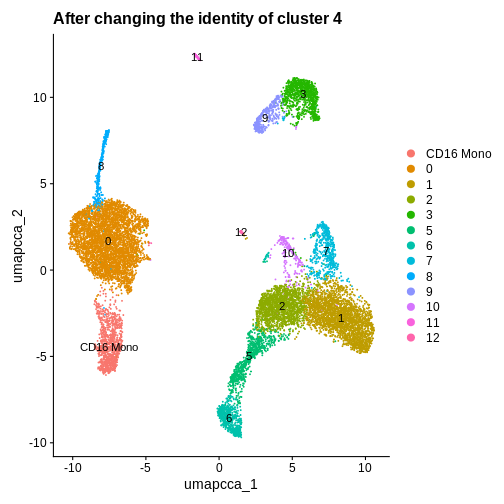
# I happen to know that the cells in cluster 4 are CD16 monocytes - lets rename this cluster
# Idents(ifnb.filtered) # Let's look at the identities of our cells at the moment
R
ifnb.filtered <- RenameIdents(ifnb.filtered, '4' = 'CD16 Mono') # Let's rename cells in cluster 4 with a new cell type label
# Idents(ifnb.filtered) # we can take a look at the cell identities again
R
DimPlot(ifnb.filtered, reduction = "umap.cca", label = T) +
  ggtitle("After changing the identity of cluster 4")
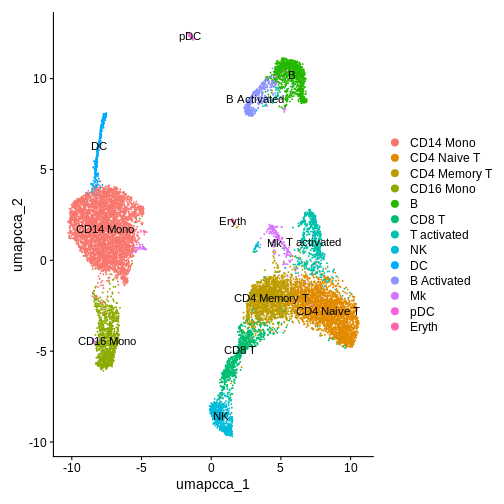
Step 2: Set the identity of our clusters to the annotations provided
R
Idents(ifnb.filtered) <- ifnb.filtered@meta.data$seurat_annotations
# Idents(ifnb.filtered)
R
DimPlot(ifnb.filtered, reduction = "umap.cca", label = T)
If you want to perform cell-type identification on your own data when you don’t have a ground-truth, using automatic cell type annotation methods can be a good starting point. This approach is discussed in more detail in the Intro to scRNA-seq workshop material.
Challenge
Automated Cell Type Annotation
R
# Load reference data
# Blood & immune lineages
ref.set <- celldex::BlueprintEncodeData()
ifnb.v4 <- JoinLayers(ifnb.filtered)
sce.ifnb.filtered <- as.SingleCellExperiment(ifnb.v4)
sce.ifnb.filtered <- logNormCounts(sce.ifnb.filtered)
pred.cnts <- SingleR(
test = sce.ifnb.filtered,
ref = ref.set,
labels = ref.set$label.main
)
lbls.keep <- table(pred.cnts$labels)>10
# Add SingleR labels to Seurat metadata
ifnb.filtered$SingleR.labels <- sce.ifnb.filtered$SingleR.labels
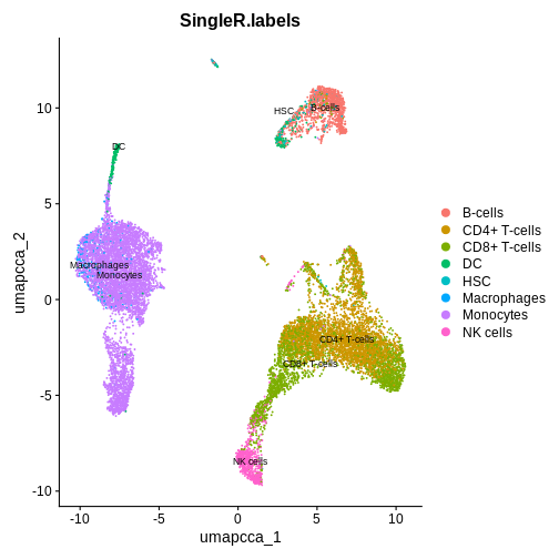
ifnb.filtered$SingleR.labels <- ifelse(lbls.keep[pred.cnts$labels], pred.cnts$labels, 'Other')
# Run UMAP (based on PCA)
ifnb.filtered <- RunUMAP(ifnb.filtered, dims = 1:20)
DimPlot(ifnb.filtered, reduction='umap.cca', group.by='SingleR.labels', label = TRUE, label.size = 3 )
Step 3: Find differentially expressed genes (DEGs) between our two conditions, using CD16 Mono cells as an example
R
# Make another column in metadata showing what cells belong to each treatment group (This will make more sense in a bit)
ifnb.filtered$celltype.and.stim <- paste0(ifnb.filtered$seurat_annotations, '_', ifnb.filtered$stim)
# (ifnb.filtered@meta.data)
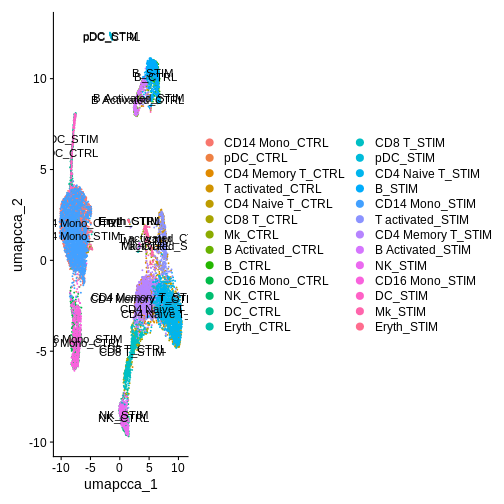
Idents(ifnb.filtered) <- ifnb.filtered$celltype.and.stim
DimPlot(ifnb.filtered, reduction = "umap.cca", label = T) # each cluster is now made up of two labels (control or stimulated)
R
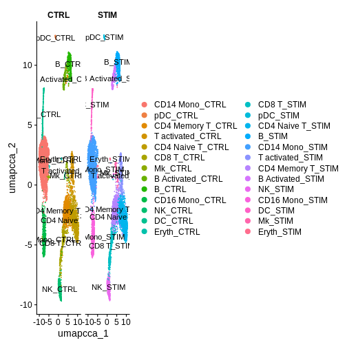
DimPlot(ifnb.filtered, reduction = "umap.cca",
        label = T, split.by = "stim") # Lets separate by condition to see what we've done a bit more clearly
We’ll now leverage these new identities to compare DEGs between our treatment groups
R
treatment.response.CD16 <- FindMarkers(ifnb.filtered, ident.1 = 'CD16 Mono_STIM',
                                       ident.2 = 'CD16 Mono_CTRL')
head(treatment.response.CD16) # These are the genes that are upregulated in the stimulated versus control group
OUTPUT
p_val avg_log2FC pct.1 pct.2 p_val_adj
IFIT1 1.379187e-176 5.834216 1.000 0.094 1.938172e-172
ISG15 6.273887e-166 5.333771 1.000 0.478 8.816694e-162
IFIT3 1.413978e-164 4.412990 0.992 0.314 1.987063e-160
ISG20 6.983755e-164 4.088510 1.000 0.448 9.814270e-160
IFITM3 1.056793e-161 3.191513 1.000 0.634 1.485111e-157
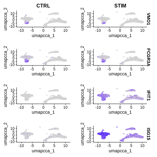
IFIT2 7.334976e-159 4.622453 0.974 0.162 1.030784e-154Step 4: Lets plot conserved features vs DEGs between conditions
R
FeaturePlot(ifnb.filtered, reduction = 'umap.cca',
            features = c('VMO1', 'FCGR3A', 'IFIT1', 'ISG15'),
            split.by = 'stim', min.cutoff = 'q10')
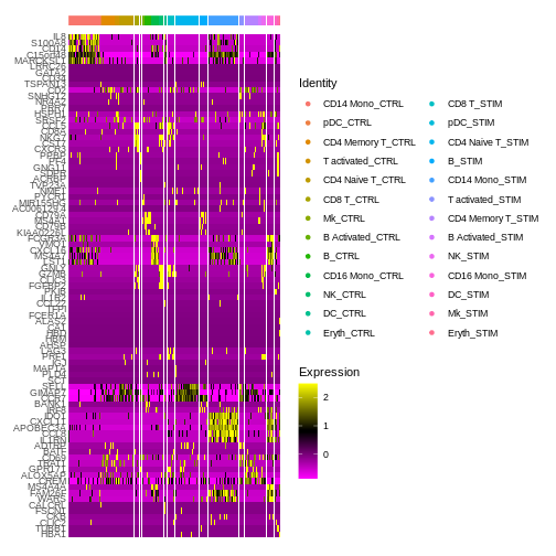
Step 5: Create a Heatmap to visualise DEGs between our two conditions + cell types
R
# Find upregulated genes in each group (cell type and condition)
ifnb.treatVsCtrl.markers <- FindAllMarkers(ifnb.filtered,
                                          only.pos = TRUE)
R
saveRDS(ifnb.treatVsCtrl.markers, "ifnb_stimVsCtrl_markers.rds")
If the top code block takes too long to run - you can download the rds file of the output using the code below:
Seurat’s in-built heatmap function can be quite messy and hard to interpret sometimes (we’ll learn how to make better and clearer custom heatmaps using the pheatmap package from our Seurat expression data later on).
R
ifnb.treatVsCtrl.markers <- readRDS(url("https://github.com/manveerchauhan/Seurat_DE_Workshop/raw/refs/heads/main/ifnb_stimVsCtrl_markers.rds"))

top5 <- ifnb.treatVsCtrl.markers %>%
  group_by(cluster) %>%
  dplyr::filter(avg_log2FC > 1) %>%
  slice_head(n = 5) %>%
  ungroup()

DEG.heatmap <- DoHeatmap(ifnb.filtered, features = top5$gene,
          label = FALSE)

DEG.heatmap
- QC filtering removes low-quality cells (e.g., low gene count or high mitochondrial %).
- Integration corrects sample-to-sample variation so cells group by biology, not by batch.
- Harmony and CCA both align shared cell states but use different mathematical strategies.