Differential Expression using a pseudobulk approach and DESeq2
Last updated on 2025-12-02 | Edit this page
Estimated time: 12 minutes
Overview
Questions
- Why aggregate to pseudobulk instead of testing each cell?
- How does donor act as the biological replicate in DESeq2?
- When do pseudobulk and single-cell DE agree or disagree, and why (e.g., zero inflation, composition, variance models)?
- What minimum sampling per group (cells per donor, donors per group) is sensible before aggregating?
Objectives
- Attach donor IDs to cells and create pseudobulk matrices with AggregateExpression().
- Run DESeq2 from Seurat via FindMarkers(test.use=“DESeq2”) on pseudobulk objects.
- Inspect and interpret key outputs (adjusted p-values, log2FC) and compare to single-cell DE.
- Visualize consensus/unique DEGs and make a publication-ready heatmap with pheatmap.
- Recognize pitfalls (uneven donor coverage, tiny groups, composition shifts) and report limitations.
OUTPUT
Modularity Optimizer version 1.3.0 by Ludo Waltman and Nees Jan van Eck

Number of nodes: 13548
Number of edges: 521570

Running Louvain algorithm...
Maximum modularity in 10 random starts: 0.9002
Number of communities: 13
Elapsed time: 1 seconds
Step 1: We need to import sample information for each cell from the original paper
Have a look at the ifnb.filtered seurat metadata, can you spot what we’ve done here?
R
# defining a function here to retrieve that information (code from https://satijalab.org/seurat/articles/de_vignette)
loadDonorMetadata <- function(seu.obj){
  # load the inferred sample IDs of each cell
  ctrl <- read.table(url("https://raw.githubusercontent.com/yelabucsf/demuxlet_paper_code/master/fig3/ye1.ctrl.8.10.sm.best"), head = T, stringsAsFactors = F)
  stim <- read.table(url("https://raw.githubusercontent.com/yelabucsf/demuxlet_paper_code/master/fig3/ye2.stim.8.10.sm.best"), head = T, stringsAsFactors = F)
  info <- rbind(ctrl, stim)

  # rename the cell IDs by substituting the '-' into '.'
  info$BARCODE <- gsub(pattern = "\\-", replacement = "\\.", info$BARCODE)

  # only keep the cells with high-confidence sample ID
  info <- info[grep(pattern = "SNG", x = info$BEST), ]

  # remove cells with duplicated IDs in both ctrl and stim groups
  info <- info[!duplicated(info$BARCODE) & !duplicated(info$BARCODE, fromLast = T), ]

  # now add the sample IDs to ifnb
  rownames(info) <- info$BARCODE
  info <- info[, c("BEST"), drop = F]
  names(info) <- c("donor_id")
  seu.obj <- AddMetaData(seu.obj, metadata = info)

  # remove cells without donor IDs
  seu.obj$donor_id[is.na(seu.obj$donor_id)] <- "unknown"
  seu.obj <- subset(seu.obj, subset = donor_id != "unknown")

  return(seu.obj)
}

ifnb.filtered <- loadDonorMetadata(ifnb.filtered)
#ifnb.filtered@meta.data
Step 2: Aggregate our counts based on treatment group, cell-type, and donor id
Collapsing our single-cell matrix in this manner is referred to as creating a ‘pseudo-bulk’ count matrix.. We’re making a condensed count matrix that looks more like a bulk matrix so that we can use bulk differential expression algorithms like DESeq2. We can see this clearly when we have a look at the ifnb.pseudbulk.df we make in the following code block.
R
ifnb.pseudobulk <- AggregateExpression(ifnb.filtered, assays = "RNA",
                                   group.by = c("stim", "donor_id", "seurat_annotations"),
                                   return.seurat = TRUE)
OUTPUT
Centering and scaling data matrixR
## Centering and scaling data matrix
# If you want the pseudobulk matrix as a dataframe you can do this:
ifnb.pseudobulk.df <- AggregateExpression(ifnb.filtered, assays = "RNA",
                                          group.by = c("stim", "donor_id", "seurat_annotations")) %>%
  as.data.frame()
We can view the top rows here:
R
head(ifnb.pseudobulk.df)
Step 3: Perform Differential Expression using DESeq2
Just like before, lets make a new column containing the cell type and treatment group before DE with DESeq2. We do this so that we can leverage the Idents() function combined with the FindMarkers function.
To use DESeq2 in older versions of Seurat (prior to v5) we would have to perform a myriad of convoluted data wrangling steps to convert our Seurat pseudobulk matrix into a format compatible with DESeq2 (or whatever bulk DE package being used). Fortunately in Seurat v5, these different bulk DE algorithms/packages have been wrapped into the FindMarker() functions - simplifying pseudobulk DE approaches immensely.
It is worth taking a look at the Seurat DE vignette on your own to see the other pseudobulk DE methods you can use. Do keep in mind that to use some of the DE tests, you need to install that package and load it as a library separately to Seurat, as we’ve done here with DESeq2 at the start.
R
ifnb.pseudobulk$celltype.and.stim <- paste(ifnb.pseudobulk$seurat_annotations, ifnb.pseudobulk$stim, sep = "_")
Idents(ifnb.pseudobulk) <- "celltype.and.stim"


# Lets run a DEG test between treated and control CD 16 monocytes using the same FindMarkers function but with DESeq2
treatment.response.CD16.pseudo <- FindMarkers(object = ifnb.pseudobulk,
                                      ident.1 = 'CD16 Mono_STIM',
                                      ident.2 = 'CD16 Mono_CTRL',
                                      test.use = "DESeq2")
OUTPUT
converting counts to integer modeOUTPUT
gene-wise dispersion estimatesOUTPUT
mean-dispersion relationshipOUTPUT
final dispersion estimatesR
head(treatment.response.CD16.pseudo)
OUTPUT
               p_val avg_log2FC pct.1 pct.2     p_val_adj
IFIT3  1.564083e-134   4.601427     1     1 2.198006e-130
IFIT2   2.122691e-84   4.613021     1     1  2.983017e-80
ISG20   1.401656e-81   4.038272     1     1  1.969747e-77
DDX58   1.366535e-73   3.448721     1     1  1.920392e-69
NT5C3A  5.127048e-66   3.942571     1     1  7.205040e-62
OASL    1.186412e-63   4.025025     1     1  1.667265e-59
R
# How are we able to use the same findmarkers function here?
head(Cells(ifnb.pseudobulk)) # our 'cells' are no longer barcodes, but have been renamed according to stim-donor-annotation when we aggregated our data earlier
OUTPUT
[1] "CTRL_SNG-101_CD14 Mono"    "CTRL_SNG-101_CD4 Naive T"
[3] "CTRL_SNG-101_CD4 Memory T" "CTRL_SNG-101_CD16 Mono"
[5] "CTRL_SNG-101_B"            "CTRL_SNG-101_CD8 T"
Step 4: Assessing differences between our pseudbulk DEGs and single-cell DEGs
First lets take a look at the DEG dataframes we made for both.
Having a look at them, can you identify any differences? Can you think of any underlying reasons behind those differences?
Hint: Look at the p_val and p_val_adj columns.
R
head(treatment.response.CD16)
OUTPUT
               p_val avg_log2FC pct.1 pct.2     p_val_adj
IFIT1  1.379187e-176   5.834216 1.000 0.094 1.938172e-172
ISG15  6.273887e-166   5.333771 1.000 0.478 8.816694e-162
IFIT3  1.413978e-164   4.412990 0.992 0.314 1.987063e-160
ISG20  6.983755e-164   4.088510 1.000 0.448 9.814270e-160
IFITM3 1.056793e-161   3.191513 1.000 0.634 1.485111e-157
IFIT2  7.334976e-159   4.622453 0.974 0.162 1.030784e-154
R
head(treatment.response.CD16.pseudo)
OUTPUT
               p_val avg_log2FC pct.1 pct.2     p_val_adj
IFIT3  1.564083e-134   4.601427     1     1 2.198006e-130
IFIT2   2.122691e-84   4.613021     1     1  2.983017e-80
ISG20   1.401656e-81   4.038272     1     1  1.969747e-77
DDX58   1.366535e-73   3.448721     1     1  1.920392e-69
NT5C3A  5.127048e-66   3.942571     1     1  7.205040e-62
OASL    1.186412e-63   4.025025     1     1  1.667265e-59
Next let’s take a look at the degree of overlap between the actual DEGs in both approaches.
To help with this, I’m just going to define a couple helper functions below.
R
Merge_DEG_dataframes <- function(pseudobulk.de,
                                 singlecell.de){
  names(pseudobulk.de) <- paste0(names(pseudobulk.de), ".bulk")
  pseudobulk.de$gene <- rownames(pseudobulk.de)

  names(singlecell.de) <- paste0(names(singlecell.de), ".sc")
  singlecell.de$gene <- rownames(singlecell.de)

  merge_dat <- merge(singlecell.de, pseudobulk.de, by = "gene")
  merge_dat <- merge_dat[order(merge_dat$p_val.bulk), ]

  return(merge_dat)
}
Visualise_Overlapping_DEGs <- function(pseudobulk.de,
                                       singlecell.de){

  merge_dat <- Merge_DEG_dataframes(pseudobulk.de,
                                    singlecell.de)

  # Number of genes that are marginally significant in both; marginally significant only in bulk; and marginally     significant only in single-cell
  common <- merge_dat$gene[which(merge_dat$p_val_adj.bulk < 0.05 &
                                   merge_dat$p_val_adj.sc < 0.05)]
  only_sc <- merge_dat$gene[which(merge_dat$p_val_adj.bulk > 0.05 &
                                    merge_dat$p_val_adj.sc < 0.05)]
  only_pseudobulk <- merge_dat$gene[which(merge_dat$p_val_adj.bulk < 0.05 &
                                      merge_dat$p_val_adj.sc > 0.05)]

  # Create a dataframe to plot overlaps
  overlap.info <- data.frame(
    category = c("Common",
                 "Only in single-cell",
                 "Only in pseudobulk"),
    count = c(length(common), length(only_sc), length(only_pseudobulk))
  )

  overlap.info$category <- factor(overlap.info$category,
                                  levels = c("Common",
                                             "Only in single-cell",
                                             "Only in pseudobulk"))
  # Create the bar plot
  overlap.bar.plt <- ggplot(overlap.info, aes(x = category, y = count, fill = category)) +
    geom_bar(stat = "identity") +
    geom_text(aes(label = count), vjust = -0.5, size = 4) +
    theme_minimal() +
    labs(title = "Number of Overlapping and Unique DEGs from Single-Cell and Pseudobulk Tests",
         x = "",
         y = "Number of Genes") +
    theme(legend.position = "none",
          axis.text.x = element_text(angle = 45, hjust = 1))

  return(overlap.bar.plt)
}
Let’s use the helper functions above to plot and view the overlap/agreement between our pseudobulk versus single-cell approaches
R
merged_deg_data <- Merge_DEG_dataframes(pseudobulk.de = treatment.response.CD16.pseudo,
                                        singlecell.de = treatment.response.CD16)
merged_deg_data %>%
  dplyr::select(gene,
                p_val.sc, p_val.bulk,
                p_val_adj.sc, p_val_adj.bulk) %>%
  head(10)
OUTPUT
       gene      p_val.sc    p_val.bulk  p_val_adj.sc p_val_adj.bulk
2866  IFIT3 1.413978e-164 1.564083e-134 1.987063e-160  2.198006e-130
2865  IFIT2 7.334976e-159  2.122691e-84 1.030784e-154   2.983017e-80
2992  ISG20 6.983755e-164  1.401656e-81 9.814270e-160   1.969747e-77
1626  DDX58 2.340153e-109  1.366535e-73 3.288617e-105   1.920392e-69
4129 NT5C3A 5.806396e-117  5.127048e-66 8.159728e-113   7.205040e-62
4185   OASL 5.497910e-147  1.186412e-63 7.726213e-143   1.667265e-59
4544 PLSCR1 6.905174e-116  3.783863e-61 9.703841e-112   5.317463e-57
3859 MYL12A  2.476988e-83  7.623767e-61  3.480912e-79   1.071368e-56
2859  IFI35  4.701828e-99  2.527378e-58  6.607479e-95   3.551724e-54
2661  HERC5  1.578848e-92  1.829060e-56  2.218755e-88   2.570378e-52
R
# How many DEGs overlap between our two methods? Is there anything in the merged_deg_data frame that stands out to you?
overlap.bar.plt <- Visualise_Overlapping_DEGs(pseudobulk.de = treatment.response.CD16.pseudo,
                                              singlecell.de = treatment.response.CD16)

overlap.bar.plt
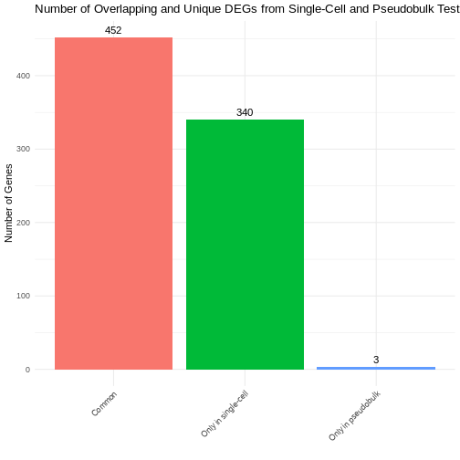
Can you explain why we’re seeing the discrepancies we see between the two methods here?
Step 5: Investigate the differences between pseudobulk DE and single-cell DE closer
Let’s create lists of genes in each of our categories first
R
common <- merged_deg_data$gene[which(merged_deg_data$p_val.bulk < 0.05 &
                                       merged_deg_data$p_val.sc < 0.05)]
only_sc <- merged_deg_data$gene[which(merged_deg_data$p_val.bulk > 0.05 &
                                        merged_deg_data$p_val.sc < 0.05)]
only_pseudobulk <- merged_deg_data$gene[which(merged_deg_data$p_val.bulk < 0.05 &
                                          merged_deg_data$p_val.sc > 0.05)]
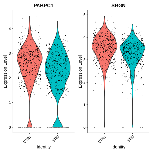
Now I want to look at the expression of genes that only appear in our sc deg test and not in our pseudobulk deg test I’ve picked two genes from the ‘only_sc’ variable we just defined
R
# create a new column to annotate sample-condition-celltype in the single-cell dataset
ifnb.filtered$donor_id.and.stim <- paste0(ifnb.filtered$stim, "-", ifnb.filtered$donor_id)
Idents(ifnb.filtered) <- "celltype.and.stim"

# Explore some genes that only appear in the sc deg test---
VlnPlot(ifnb.filtered, features = c("PABPC1", "SRGN"),
        idents = c("CD16 Mono_CTRL", "CD16 Mono_STIM"),
        group.by = "stim")
R
VlnPlot(ifnb.filtered, features = c("PABPC1", "SRGN"),
        idents = c("CD16 Mono_CTRL", "CD16 Mono_STIM"),
        group.by = "donor_id.and.stim", ncol = 1)
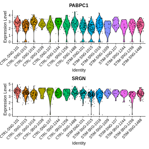
How would you interpret the plots above? What does this tell you about some of the pitfalls of single-cell DE approaches?
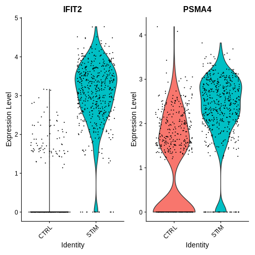
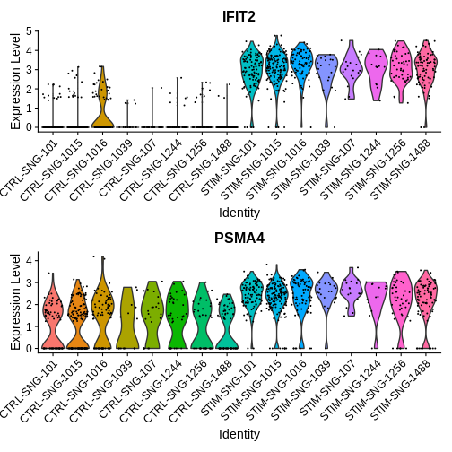
Now lets take a look at some genes that show agreement across both sc and pseudobulk deg tests
R
VlnPlot(ifnb.filtered, features = c("IFIT2", "PSMA4"),
        idents = c("CD16 Mono_CTRL", "CD16 Mono_STIM"),
        group.by = "stim")
R
VlnPlot(ifnb.filtered, features = c("IFIT2", "PSMA4"),
        idents = c("CD16 Mono_CTRL", "CD16 Mono_STIM"),
        group.by = "donor_id.and.stim", ncol = 1)
Step 6: Creating our own custom visualisations for DEG analysis between cell-types in two different experimental groups
So far, we’ve been using functions wrapped within Seurat to plot and visualise our data. But we’re not limited to those functions. Let’s use the pheatmap (‘pretty heatmap’) package to visualise our DEGs with adjusted p values < 0.05.
First lets look at our significant DEGs as defined by our pseudobulk approach
R
CD16.sig.markers <- treatment.response.CD16.pseudo %>%
  dplyr::filter(p_val_adj < 0.05) %>%
  dplyr::mutate(gene = rownames(.))
This is how we can pull our average (scaled) pseudobulk expression values from our seurat obj:
R
ifnb.filtered$celltype.stim.donor_id <- paste0(ifnb.filtered$seurat_annotations, "-",
                                               ifnb.filtered$stim, "-", ifnb.filtered$donor_id)
Idents(ifnb.filtered) <- "celltype.stim.donor_id"

all.sig.avg.Expression.mat <- AverageExpression(ifnb.filtered,
                         features = CD16.sig.markers$gene,
                         layer = 'scale.data')
OUTPUT
As of Seurat v5, we recommend using AggregateExpression to perform pseudo-bulk analysis.
This message is displayed once per session.
R
## As of Seurat v5, we recommend using AggregateExpression to perform pseudo-bulk analysis.
## This message is displayed once per session.

# View(all.sig.avg.Expression.mat %>%
#  as.data.frame())
Now lets make sure we’re only using data from the CD16 cell type
R
CD16.sig.avg.Expression.mat <- all.sig.avg.Expression.mat$RNA %>%
  as.data.frame() %>%
  dplyr::select(starts_with("CD16 Mono"))

# View(CD16.sig.avg.Expression.mat)
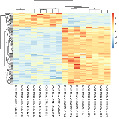
Let’s finally view our heatmap with averaged pseudobulk scaled expression values for our signficant DEGs
R
pheatmap::pheatmap(CD16.sig.avg.Expression.mat,
         cluster_rows = TRUE,
         show_rownames = FALSE,
         border_color = NA,
         fontsize = 10,
         scale = "row",
         fontsize_row = 10,
         height = 20)
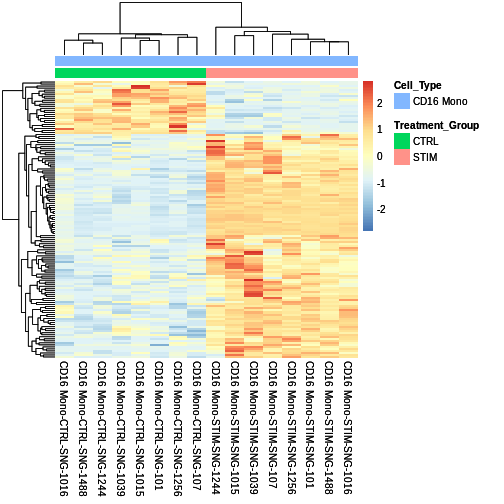
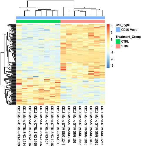
The cool thing about pheatmap is that we can customise our heatmap with added metadata
R
cluster_metadata <- data.frame(
  row.names = colnames(CD16.sig.avg.Expression.mat)
) %>%
  dplyr::mutate(
    Cell_Type = "CD16 Mono",
    Treatment_Group = ifelse(str_detect(row.names(.), "STIM|CTRL"),
                      str_extract(row.names(.), "STIM|CTRL")))

sig.DEG.heatmap <- pheatmap::pheatmap(CD16.sig.avg.Expression.mat,
         cluster_rows = TRUE,
         show_rownames = FALSE,
         annotation = cluster_metadata[, c("Treatment_Group", "Cell_Type")],
         border_color = NA,
         fontsize = 10,
         scale = "row",
         fontsize_row = 10,
         height = 20,
         annotation_names_col = FALSE)

sig.DEG.heatmap
Lets save our heatmap using the grid library (very useful package!) Code from: https://stackoverflow.com/questions/43051525/how-to-draw-pheatmap-plot-to-screen-and-also-save-to-file
R
save_pheatmap_pdf <- function(x, filename, width=7, height=7) {
   stopifnot(!missing(x))
   stopifnot(!missing(filename))
   pdf(filename, width=width, height=height)
   grid::grid.newpage()
   grid::grid.draw(x$gtable)
   dev.off()
}

save_pheatmap_pdf(sig.DEG.heatmap, "sig_DEG_pseudo.pdf")
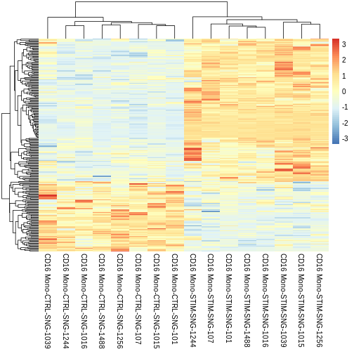
Challenge
Do the same thing with significant DEGs from the sc approach. Do you see any differences?
Run the same code as above but with the
treatment.response.CD16 variable instead of
treatment.response.CD16.pseudo variable.
R
CD16.sig.markers <- treatment.response.CD16 %>%
  dplyr::filter(p_val_adj < 0.05) %>%
  dplyr::mutate(gene = rownames(.))

ifnb.filtered$celltype.stim.donor_id <- paste0(ifnb.filtered$seurat_annotations, "-",
                                               ifnb.filtered$stim, "-", ifnb.filtered$donor_id)
Idents(ifnb.filtered) <- "celltype.stim.donor_id"

all.sig.avg.Expression.mat <- AverageExpression(ifnb.filtered,
                         features = CD16.sig.markers$gene,
                         layer = 'scale.data')

## As of Seurat v5, we recommend using AggregateExpression to perform pseudo-bulk analysis.
## This message is displayed once per session.

# View(all.sig.avg.Expression.mat %>%
#  as.data.frame())

CD16.sig.avg.Expression.mat <- all.sig.avg.Expression.mat$RNA %>%
  as.data.frame() %>%
  dplyr::select(starts_with("CD16 Mono"))

# View(CD16.sig.avg.Expression.mat)

pheatmap::pheatmap(CD16.sig.avg.Expression.mat,
         cluster_rows = TRUE,
         show_rownames = FALSE,
         border_color = NA,
         fontsize = 10,
         scale = "row",
         fontsize_row = 10,
         height = 20)
R
cluster_metadata <- data.frame(
  row.names = colnames(CD16.sig.avg.Expression.mat)
) %>%
  dplyr::mutate(
    Cell_Type = "CD16 Mono",
    Treatment_Group = ifelse(str_detect(row.names(.), "STIM|CTRL"),
                      str_extract(row.names(.), "STIM|CTRL")))

sig.DEG.heatmap <- pheatmap::pheatmap(CD16.sig.avg.Expression.mat,
         cluster_rows = TRUE,
         show_rownames = FALSE,
         annotation = cluster_metadata[, c("Treatment_Group", "Cell_Type")],
         border_color = NA,
         fontsize = 10,
         scale = "row",
         fontsize_row = 10,
         height = 20,
         annotation_names_col = FALSE)

sig.DEG.heatmap
You have now completed the workshop!
Hopefully you’ve found this workshop useful and you’re now feeling more confident about using different integration and differential expression approaches in single-cell data analysis.
What kind of analyses do you think we can do next after obtaining a list of differentially expressed genes (DEGs) for each cell type and treatment groups?
- Collapse single-cell counts to pseudobulk per donor × condition × cell type.
- Compare single-cell DE vs pseudobulk DE.